C O D E: DigitDemo v1.0

Description: This code package contains an interactive demo of Gibbs sampling, mean-field reconstruction and classification for restricted Boltzmann machines trained using four different inductive principles including stochastic maximum likelihood (SML), contrastive divergence (CD), ratio matching (RM) and pseudo-likelihood (PL). The MNIST data set was used as training data. 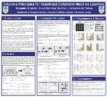See our AISTATS 2010 paper Inductive Principles for Restricted Boltzmann Machine Learning for details. Note that this demo uses trained models and does not include code for learning.

System Requirements:

Because of differences in GUI handling in different versions of Matlab, this code package requires Matlab 7.2 or higher to function properly.
The GUI was designed for a 1280x1024 screen resolution. Some GUI elements may not automatically re-position themselves nicely on smaller screens.

Download: DigitDemo.zip (11.7MB)

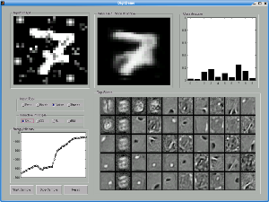
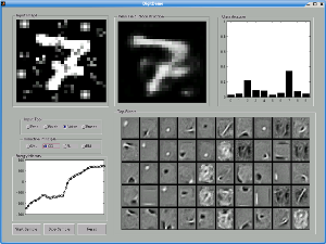
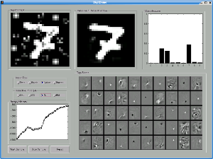
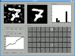
Example: This example shows the mean-field reconstruction and classification of a seven with noise added. We see that SML and CD have significantly degraded mean-field reconstructions in the presence of noise compared to RM and PL. All of the models make the correct classification, but RM is much more certain that the image is a seven.

SML	CD
PL	RM

Usage:

Launch the GUI by entering "DigitDemo" at the Matlab prompt.

You can draw in the "Input Image" panel by clicking and dragging with the mouse. You can select different input tools from the "Input Tool" control including:

The Pen Tool: Sets 2x2 blocks to solid white
The Brush Tool: Sets 3x3 blocks to white with a soft fall-off
The Noise Tool: Adds 3x3 blocks of white noise to the image
The Eraser Tool: Set 2x2 blocks to solid black

You can erase the input image by clicking on the "Reset" button.

You can select RBM models trained using different inductive principles using the "Inductive Principle" control. You can switch between models at any time, including while the Gibbs sampler is running. The inductive principles include:

SML: Stochastic Maximum Likelihood. Also called Persistent Contrastive Divergence or PCD
CD: Contrastive Divergence
PL: Pseudo-Likelihood
RM: Ratio Matching

As you draw, the GUI displays the mean-field reconstruction in the "Mean-Field Reconstruction" panel for the model currently selected using the "Inductive Principle" control. The mean-field reconstruction is obtained by going from the input image to the hidden unit activations and back to the input image. It is often able to fill-in gaps in digits as well as remove noise.

A linear classification model also attempts to predict the digit you are drawing in real time as you draw it. A separate classifier was trained using RBM hidden unit activations as input for each of the four inductive principles. The results are displays as a distribution over the digits 0 to 9 in the "Classification" panel.

The un-normalized free energy of the input image under the currently selected model is displayed in real time in the "Free Energy History" panel. Relative changes in free energy correspond to changes in log probability of the input. Remember that lower energy corresponds to higher probability.

The most active hidden units are also displayed for the currently selected model as filters (matrix of all weights leaving a hidden unit) and are updated in real time as you draw. The filters are a representation of the input features that each hidden unit has learned to pay attention to. The degree to which these filters are active is the input to the classifier, while the mean-field reconstruction of the input image is obtained by a hidden-unit-activation weighted linear combination of the filters.

You can run a Gibbs sampler initialized from the current input image at any time by clicking the "Start Sample" button. You can stop the sampler by clicking the "Stop Sample" button. The Gibbs sampler samples binary values for the input image pixels. The soft visible unit probabilities are instead displayed in the "Mean-Field Reconstruction" panel to reduce noise in the visualization. All of the above outputs (classification, energy history, filters) are updated while the Gibbs sampler runs. You can also switch between trained models using the "Inductive Principles" control while the sampler runs.