Justin's Graphical Models / Conditional Random Field Toolbox
This is a Matlab/C++ "toolbox" of code for learning and inference
with graphical models. It is focused on parameter learning using
marginalization in the high-treewidth setting. Though the code is,
in principle, domain independent, I've developed it with vision
problems in mind, particularly for learning Conditional Random
Fields (CRFs). This means that the code is A) efficient (all the inference algorithms are implemented in C++) and B) can handle arbitrary graph structures.
There are, at present, a bunch of limitations:
All the inference algorithms are for marginal inference. No MAP inference, at all.
The code handles pairwise graphs only
All variables must have the same number of possible values.
For tree-reweighted belief propagation, a single edge appearance probability must be used for all edges
For vision, these are usually no big deal. In other domains, though, these might be showstoppers.
Size: (non-comment lines of code)
Matlab: 4204
C++: 1322
The code can be downloaded here. Note that
it includes a set of binaries for various things for efficiency. I've included binaries for 64-bit OS X, 64-bit linux, and 64-bit Windows. (Many thanks to David Klein and Alexei Skurikhin for providing Windows Binaries!) If you compile the code for a different platform, please email me the binaries so they could be included for others.
Version 2 (Jan 4 2012): JGMT2.zip (Obsolete)
Bugfixes, binaries for linux, new generic train_crf inferface,
multithreaded back-TRW switch from Eigen 2 to Eigen 3.
Version 3 (Sep 9 2013): JGMT3.zip (Obsolete) More windows binaries, small bugfix for HoG features
Version 4 (April 20 2015): JGMT4.zip minor bugfix to adapt to changes in external libraries.
Windows Binaries
If you are interested in using the code on Windows, Alexei Skurikhin has provided a set of binaries. Most of these are provided with the main code above, however, there are also special binaries to use openMP multithreading, and some details on how to compile if the binaries do not work on your system.
Many loss functions return the marginals that were computed to arrive at the loss. However, the pseudolikelihood (the point of which is that inference is not necessary) does not do this.
The code has a particular convention for unlabled variables. Specifically, this toolbox uses a label of 0 to represent unlabelled variables. Note that this is not the same thing as a "background" label. If you have fully-labeled binary data, you should use labels of 1 and 2, and reserve 0 only for missing data. If you mistakenly use labels of 0 and 1, the model will happily learn to predict "1" everywhere.
Use the Differentiation methods (back-TRW or implicit differentiation) to calculate parameter gradients by providing your own loss functions. Do everything else on your own.
Use the Loss methods (E.M., implicit_loss) to calculate parameter gradients by providing a true vector x and a loss name (univariate likelihood, clique likelihood, etc.) Unlike the above usages, these methods explicitly consider the conditional learning setting where one has an input and an output.
Use the CRF methods to do almost everything (deal with parameter
ties for a specific type of model, etc.) These methods consider
specific classes of CRFs and given and input, output, loss function,
inference method, etc. give the parameter gradient. Employing this
gradient in a learning framework is straightforward.
>> wget http://dags.stanford.edu/data/iccv09Data.tar.gz
Resolving dags.stanford.edu...
Connecting to dags.stanford.edu
HTTP request sent, awaiting response... 200 OK
Length: 14727974 (14M) [application/x-gzip]
Saving to: ?iccv09Data.tar.gz?

100%[======================================>] 14,727,974  3.03M/s   in 6.7s

2011-12-17 18:23:42 (2.10 MB/s) - ?iccv09Data.tar.gz? saved [14727974/14727974]

>> tar -xvf iccv09Data.tar.gz
iccv09Data/horizons.txt
iccv09Data/images/
iccv09Data/images/0000051.jpg
iccv09Data/images/0000059.jpg
iccv09Data/images/0000072.jpg
[...]
iccv09Data/labels/9005273.layers.txt
iccv09Data/labels/9005294.regions.txt
iccv09Data/labels/9005294.surfaces.txt
iccv09Data/labels/9005294.layers.txt
iccv09Data/README
This puts the data in a directory at ~/Datasets/iccv09Data/.
Now, start matlab. We begin with some parameter choices.
imsdir = '~/Datasets/iccv09Data/images/'; % Change this to fit your system!
labdir = '~/Datasets/iccv09Data/labels/'; % Change this to fit your system!
nvals  = 8;
rez    = .2; % how much to reduce resolution
rho    = .5; % (1 = loopy belief propagation) (.5 = tree-reweighted belief propagation)
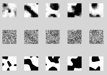
Next, we need to choose what features will be used. Here, we choose
to use the RGB intensities, and position, jointly Fourier expanded,
plus a histogram of Gaussians, computed using Piotr Dollar's toolbox.
Now, we will load the data. In the backgrounds dataset, labels are stored as a text array of
integers in the range 0-7, with negative values for unlabelled
regions. JGMT uses 0 to represent unlabelled/hidden values, so we make
this conversion when loading the data. Additionally, we reduce
resolution to 20% after computing the features. This actually
increases the accuracy of the final predictions, interpolated
back to the original resolution.
ims_names = dir([imsdir '*.jpg']);
lab_names = dir([labdir '*regions.txt']);
N = length(ims_names);
ims    = cell(N,1);
labels = cell(N,1);

fprintf('loading data and computing feature maps...\n');
parfor n=1:N
    % load data
    lab = importdata([labdir lab_names(n).name]);
    im  = double(imread(([imsdir ims_names(n).name])))/255;
    ims{n}  = im;
    labels0{n} = max(0,lab+1);

    % compute features
    feats{n}  = featurize_im(ims{n},feat_params);

    % reduce resolution for speed
    ims{n}    = imresize(ims{n}   ,rez,'bilinear');
    feats{n}  = imresize(feats{n} ,rez,'bilinear');
    labels{n} = imresize(labels0{n},rez,'nearest');

    % reshape features
    [ly lx lz] = size(feats{n});
    feats{n} = reshape(feats{n},ly*lx,lz);
end
Next, we will make the graph structure. In this dataset, the images
come in slightly different sizes. Rather than making a different
graph for each image (which would be fine if slow) we use a "hashing"
strategy to make them, then copy into an array with one per image.
model_hash = repmat({[]},1000,1000);
fprintf('building models...\n')
for n=1:N
[ly lx lz] = size(ims{n});
if isempty(model_hash{ly,lx});
model_hash{ly,lx} = gridmodel(ly,lx,nvals);
endend
models = cell(N,1);
for n=1:N
[ly lx lz] = size(ims{n});
models{n} = model_hash{ly,lx};
end
Now, we compute edge features. (This must be done here since it uses
the graph structures.) First off, we must specify what features to
use. Here, we choose a constant of one, a set of thresholds on the
difference of neighboring pixels, and "pairtype" features. In pairtype
last ones, the number of features is doubled, with the previous
features either put in the first or second half. The effect is that
vertical and horizontal edges are parameterized separately.
Next up, we split the data into a training set (80%) and a test set (20%).
fprintf('splitting data into a training and a test set...\n')
k = 1;
[who_train who_test] = kfold_sets(N,5,k);

ims_train     = ims(who_train);
feats_train   = feats(who_train);
efeats_train  = efeats(who_train);
labels_train  = labels(who_train);
labels0_train = labels0(who_train);
models_train  = models(who_train);

ims_test     = ims(who_test);
feats_test   = feats(who_test);
efeats_test  = efeats(who_test);
labels_test  = labels(who_test);
labels0_test = labels0(who_test);
models_test  = models(who_test);
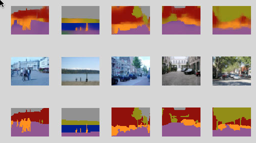
Again we make a visualization function. This takes a cell array of predicted
beliefs as input, and shows them to the screen during training. This
is totally optional, but very useful if you want to understand what
is happening in your training run.
% visualization functionfunction viz(b_i)
% here, b_i is a cell array of size nvals x nvars
M = 5;
for n=1:M
[ly lx lz] = size(ims_train{n});
subplot(3,M,n ); miximshow(reshape(b_i{n}',ly,lx,nvals),nvals);
subplot(3,M,n+ M); imshow(ims_train{n})
subplot(3,M,n+2*M); miximshow(reshape(labels_train{n},ly,lx),nvals);
end
xlabel('top: marginals middle: input bottom: labels')
drawnow
end
Now, we choose what learning method to use. Here, we choose
truncated fitting with the clique logistic loss. We use 5 iterations
of TRW inference. Here, we use 'trwpll' to indicate to use the
multithreaded TRW code. You will probably have to call
'compile_openmp' to make this work. Otherwise, you could just switch
to 'trunc_cl_trw_5', which uses the non-parallel code.
loss_spec = 'trunc_cl_trwpll_5';
Finally, we actually train the model. This takes about an hour and a
half on an 8-core machine. You should have at least 4-8GB of memory.
matlabpool 8

fprintf('training the model (this is slow!)...\n')
crf_type  = 'linear_linear';
options.viz         = @viz;
options.print_times = 0; % since this is so slow, print stuff to screen
options.gradual     = 1; % use gradual fitting
options.maxiter     = 1000;
options.rho         = rho;
options.reg         = 1e-4;
options.opt_display = 0;
p = train_crf(feats_train,efeats_train,labels_train,models_train,loss_spec,crf_type,options)

ans =

    F: [8x100 double]
    G: [64x22 double]
The result is a structure array p. It contains two matrices. The
first, F, determines the univariate potentials. Specifically, the
vector of log-potentials for node i is given by multiplying F with the
features for node i. Since there are 100 univariate features, this is
a 8x100 matrix. Similarly, G determines the log-potentials for
the edge interactions. Since there are 22 edge features and 64=8*8
pairwise values, this is a 64x22 matrix.
fprintf('get the marginals for test images...\n');
close allfor n=1:length(feats_test)
[b_i b_ij] = eval_crf(p,feats_test{n},efeats_test{n},models_test{n},loss_spec,crf_type,rho);
[ly lx lz] = size(labels_test{n});
[~,x_pred] = max(b_i,[],1);
x_pred = reshape(x_pred,ly,lx);
[ly lx lz] = size(labels0_test{n});
x = labels0_test{n};
% upsample predicted images to full resolution
x_pred = imresize(x_pred,size(x),'nearest');
E(n) = sum(x_pred(x(:)>0)~=x(x(:)>0));
T(n) = sum(x(:)>0);
[ly lx lz] = size(ims_test{n});
subplot(2,3,1)
miximshow(reshape(b_i',ly,lx,nvals),nvals);
subplot(2,3,2)
imshow(ims_test{n})
subplot(2,3,3)
miximshow(reshape(labels_test{n},ly,lx),nvals);
[ly lx lz] = size(labels0_test{n});
subplot(2,3,4)
miximshow(reshape(x_pred,ly,lx),nvals);
subplot(2,3,5)
imshow(ims_test{n})
subplot(2,3,6)
miximshow(reshape(labels0_test{n},ly,lx),nvals);
drawnow
end
fprintf('total pixelwise error on test data: %f \n', sum(E)/sum(T))
In this case, the error on test data is around 23%. Certainly not
perfect, but seems to be state of the art on this dataset currently.
Finally, for fun, I also downloaded a video of someone driving from Arlington
into Georgetown and ran the algorithm. This took about .62s per frame
to compute the features and .75s per frame to run TRW (though
inference has been optimized for learning, not test time
performance). Anyway, this gives a performance of "0.73
FPS". Not fast enough to process video in real time, but potentially
useful in a robotics application or similar