Cryptographic hashes and Perceptual hashes
My apologies, these notes are more of an outline than the prose we are used to in this course.
Non-cryptographic hashing (FNV)
Hans Peter Luns invented the first non-crypto hash (article).
Fowler–Noll–Vo, or FNV, is a very common non-cryptographic hash function created by Glenn Fowler, Landon Curt Noll, and Kiem-Phong Vo.
You can use it in python from the pyhash package.
It’s pretty straight forward. Given the hash size, there is a given prime number and an initial value that is iterated on. For a 64-bit hash, it looks like this pseudocode:
prime = 0x100000001b3

hash = 0xcbf29ce484222325
for each byte of input:
    hash  = (hash * prime) xor the_byte mod 2**64
Cryptographic Hashing
Cryptographic hash functions were first described in detail by Ralph Merkle in his 1979 PhD thesis.
Cryptographic hash functions take an digital input of any finite size and produce a fixed size output.
If x is the input, and x’ represents any single flipped bit of x, then cryptographic hashes have the property that each output bit has equal and independent probability of being a 0 or a 1.
There should be no way to predict the output of the hash from its input other than by running the actual hash function. This is often referred to pseudo-randomness. (But also note that the output is deterministic: the hash of any given input never changes.)
The three main properties of cryptographic hash functions
Pre-image resistance: It should be computationally infeasible to find a sequence of bytes that has a specific hash. That is, given hash output value \(y\), it should be hard to find an \(x\) such that \(y=h(x)\).
Second pre-image resistanceIt should be computationally infeasible to find a second sequence \(m_2\) that has the same hash as a first sequence \(m_1\). That is, given \(m_1\), it should be hard to find a \(m_2\) such that \(h(m_2)==h(m_1)\).
Collision resistance This property is sometimes call the “birthday attack”. It should be hard to find a pair of inputs \(m_x\) and \(m_y\) such that \(h(m_x)==h(m_y)\).
What’s difference between the last two properties? In the case of Second pre-image resistance, we fix \(m_1\). In the case of collision resistance, we don’t care what the two pairs are.
Some example cryptographic hash functions include: MD5, SHA-1, SHA-256, and SHA-512
Is it ok to use MD5 or SHA-1?
MD5 is still in use today, but it should no longer be used because it is now relatively straightforward to generate two blocks of data that have the same MD5 hash. That is, MD5 no longer has collision resistance.
On the other hand, there is still no publicly known attack on MD5 that will let you find a block of data with a specific MD5 hash— that is, it still is publicly considered to have pre-image resistance.
SHA-1 has been shown to no longer has collision resistance.
See the article by Garfinkel that discusses this issue.
Small block forensics
Simson Garfinkel developed a technique called small block forensics that is used in the field to overcome the time it takes to search very large drives for content. Keep in mind this is particularly useful when we are looking on a very large drive for any one file from a large set of files of interest. For example, investigators may have a large set of movies they are interested in, and they are looking at a 20TB hard drive. The goal is not to categorize every file on the 20TB drive; instead, we seek to know if the drive contains even one of the movies of interest. If that’s the case, then the investigators spend the time looking through every file, which is time consuming but now since one movie of interest was found, perhaps more will be found.
Garfinkel’s solution is to sample random sectors from the drive. Here we are basically ignoring the fact that file systems are based on clusters. Nor do we even care what file system it is. We just need to be sure that the file system is unencrypted. To prepare for this scenario, the investigator keeps a database of cryptographic hash values of interest. The hash values are not of entire movies; instead it’s a hash of every 512 byte sector of a movie of interest. For example, if a movie is 1MiB long then it has 2048 sectors. Each sector will be hashed and placed in a database. Next, the investigator selects a random sector from the drive being investigated and then determines if its hash value is in the database. If so, then the drive might contain more content of interest.
The important question is, how many sectors does the investigator need to sample from to be very sure they will detect at least one (not all, just at least one) of the sectors of interest, given that a movie of interest is contained on the drive? What do I mean by “very sure”? I mean like a good 90% of succeeding.
In particular, Simson’s states a formula for \(p\), the probability of successfully finding a sector of interest when you sample \(n\) sectors from a drive with \(N\) sectors total of which \(C\) sectors are content of interest.
In the article, there is a typo: it says the product is from “i-1” instead of “i=1”. It should be stated like so:
To explain this a little more, note that there are \(N\) sectors on the disk, and \(C\) of them are sectors of interest to us. Picking one of the \(C\) sectors is a success. Simson has us select \(n\) sectors at random. We want to know the Probability of selecting 1 or more of the \(C\) sectors if we select \(n\) sectors without replacement, one at a time. That probability is equal to 1 minus the probability of the complement. The complement is we select \(n\) sectors and never pick a sector from \(C\). So, at selection \(i=1\), the probability of not selecting a sector of interest is \(N-C\) sectors out of \(N\); i.e., it’s \(\frac{N-C}{N}\). For selection \(i=2\), we have 1 less sector on the disk to consider, so the probability is \(\frac{N-1-C}{N-1}\). For selection \(i\) it’s \(\frac{N-(i-1)-C}{N-(i-1)}.\) We need all selections to succeed, and so we must multiply the probabilities together. And don’t forget, we are in a “1 minus” situation, so we have.
which is equal to
Now let’s consider some examples that Simson provides. He says
Although the sample contains only 0.05 percent of the (Tbyte-sized) drive, there is a 98.17 percent chance of detecting 4 Mbytes of known content, provided that each of those 8,000 blocks is in the database.
Keep in mind that the hardrives use fake math. A “one terabyte” drive is not a “1 Tebibyte drive”. So, he’s saying (1 terabyte) / (500 bytes/sector) =2,000,000,000 sectors. (Yes, hard drive math is not real; we all know that sectors are always 512 bytes!)
- What’s N? 2,000,000,000 sectors.
- What’s C? 8000 sectors.
- What’s n? 0.05% *2,000,000,000 = 1,000,000
Then he says
Applying this equation to 500,000 and 250,000 randomly selected sectors, we find that the chance of detecting 4 Mbytes of known content, provided each of the 8,000 blocks is in the database, is 86.47 percent and 63.21 percent, respectively.
In these examples, \(N=2000000000\) still, and \(C=8000\) still. We are just changing up \(n\).
Perceptual Hashing
Cryptographic hashes can be great for identifying images that aren’t modified. But what if I change a few bits? Or save a jpeg as a png? the hash won’t match.
Perceptual hashes give a signature of an image, one that doesn’t change too much if the image changes. Further it’s based on the view of the image and not its data. That is, it’s converted to pixel values before the hash is taken.
The jupyter notebook I used in class is on moodle.
Here’s a link to the source of the hash library I used. Here’s some discussion of perceptual hashing.
Results from the Notebook
Here’s the visualization of the transformations in the notebook:
- Original

- Resized

- Edges

- Flip

- Gauss (1)

- Gauss (5)

- Rotate 1 degree

- Rotate 2 degree

- Rotate 15 degree

Some more plots to look at.
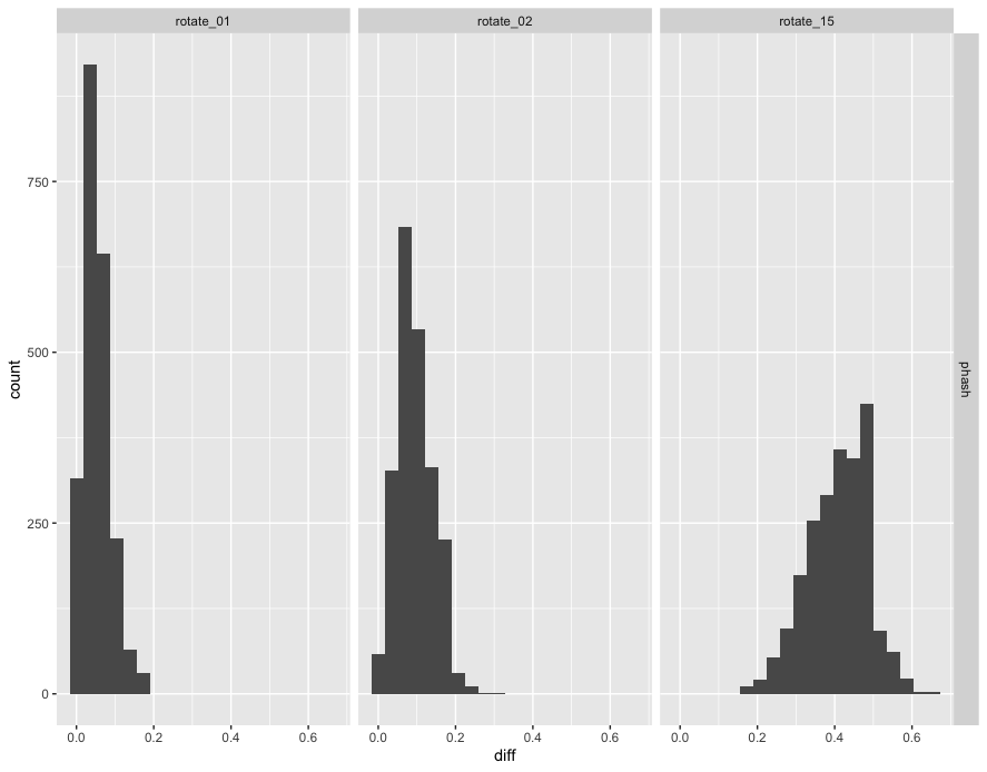
Here’s the frequency distribution (the histogram) of the hamming distance between Phash(original) and Phash(rotated). To the left on the x-axis means less difference. To the the right is great difference in phash values.
The differences in phash values tend to be larger as the rotation is greater from 01 to 02 to 15 degrees rotation.
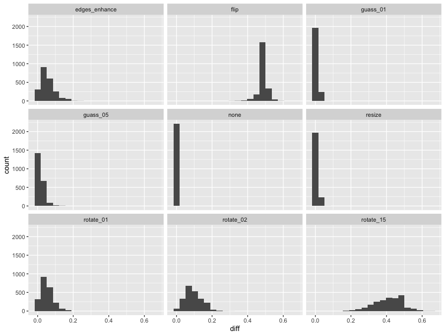
Here’s the same type of histogram for the other transformations.
Evaluation of Classifiers
The simplest classifier is a binary classifer, which determines whether something is true or false. Do I have covid or not? Is this spam email or not? Is this image contraband or not? Classifiers almost always have an error rate. Sometimes you actually have covid (it’s TRUE that you do) but the test may result in a “positive” or “negative” for covid. Sometimes you actually don’t have covid (it’s FALSE that you do) but the test may result in a “positive” or “negative” for covid. Therefore, all binary classifier have FOUR outcomes as this confusion matrix shows.
| Actual (T or F) | |||
|---|---|---|---|
| | TRUE | | FALSE | ||
| Predictions | POSITIVE | | true positive (TP) | | false positive (FP) |
| (P or N) | NEGATIVE | | false negative (FN) | | true negative (TN) |
Let’s look a little closer at the internals of how a typical binary classifier works. A prediction is output as a floating point value from 0 to 1. Zero means the classifier is very “confident” than the prediction should be negative. One means that the classifier is very confident that the prediction should be positive. And so you might get a prediction of 0.3 from a classifier.
You might be assuming right now that any prediction above a threshold of 0.5 and above becomes a TRUE and any prediction below a threshold of 0.5 is a FALSE. Well, that’s just one option. In fact, you can set the threshold to anything you wish.
At an extreme, you can set the threshold to 0, and everything will be a TRUE. As a result, you’ll never have a False Negative.
At another extreme, you can set the threshold to 1, and everything will be a FALSE. As a result, you’ll never have a False Positive.
Thresholds in between represent a trade off FNs and FPs that depends on your data set and the quality of your classifier.
Scientists use several statistical metrics to talk about these trade offs.
-
The True Positive Rate (TPR) (also called Recall) is the TP/(TP+FN). (Keep in mind this equation means “The count of all true positives in the numerator; the denominator is the count of all true positives.) It’s the fraction of all actual positives that were correctly classified to be positives.
-
The Precision is TP/(TP+FP). It is the fraction of all data classified as positive that were actual positives. (see the difference?)
-
The False Positive Rate (FPR) is FP/(FP+TN). It is the fraction of all actual negatives that were wrongly classified to be positive.
So to repeat myself using these metrics:
-
At an extreme, you can set the threshold to 0, and everything will be a TRUE. As a result, you’ll never have a False Negative. Accordingly, your TPR (or recall) will be 100%.
-
At another extreme, you can set the threshold to 1, and everything will be a FALSE. As a result, you’ll never have a False Positive. Accordingly, your FPR will be 0%.
-
If you examine a range of thresholds, then you’ll observe a range of tradeoffs.
Plotting results
Coming back to the perceptual hashes you might ask how we can relate it to the predictions and thresholds I wrote about above? Let’s review how it works. We take the p-hash value of image A, which is a series of bits, and we get the same for image B. Keep in mind the p-hash is a series of bits of length \(n\). Then we take the Hamming distance of the two hash values. The Hamming distance gives us a count of bits that differ between the two results. To make that into a prediction, we take two steps. First, we convert it to a fraction by dividing by the maximum number of bits that could be different — which is the size of the bit strings, \(n\). In this representation, two images with the same p-hash value should have no bits different and have a value of \(\frac{0}{n}=0\). Two images with different bits will have a value of \(\frac{n}{n}=1\). Therefore, we need to take a second step and set the prediction to “1 minus”. Meaning, it’s \(1-\frac{0}{n} = 1\) and \(1-\frac{n}{n}=0\).
In general, we start with \(c = Hamming( phash(A), phash(b))\) and calculate the prediction as \(=1-\frac{c}{n}\).
Ok, now that we have predictions, it’s interesting to plot TPR again FPR given a range of thresholds. The values in the TOP LEFT are the best performing results. Because there FPR is zero and TPR is one.
In this first plot, all lines in a single plot are for one algorithm; each line is a different transformation. And so the plot tells you how the specific hash changes with the transformation.
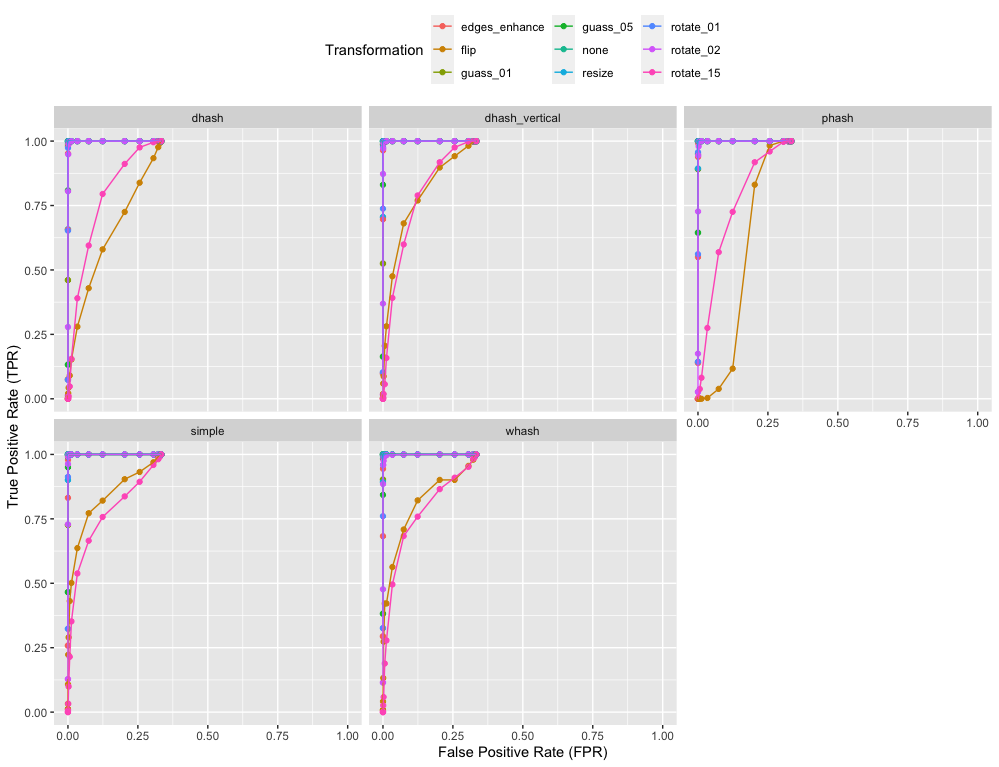
In this second plot, all lines in a single plot are for the same transformation; each line is a different algorithm. And so the plot tells you how the specific transformation affects each algorithm.
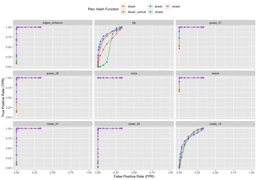
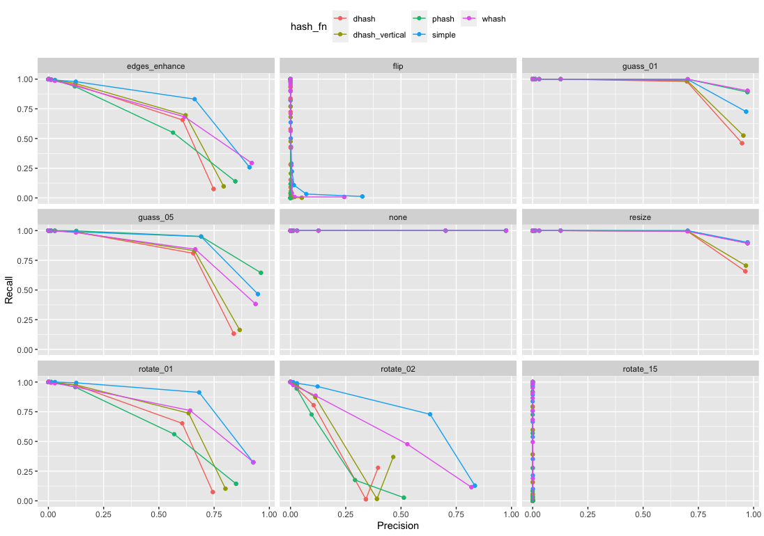
It’s also interesting to plot Precision versus Recall (i.e., Precision versus TPR). Here the values in the TOP RIGHT are best performing because there Precision is high and Recall is high.
You can see the flip and rotate 15 are not handled by these algorithms. But that small amounts of blur are handled a little better. Resizing has the least affect on the algorithms.
