[adapted from B. Ravindran's course, Fall 2005]:
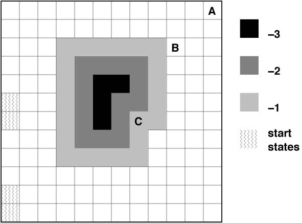
The aim of the exercise is to familiarize you with function approximation approaches. You will solve a larger version of the puddle world problem, where the gridworld is of size 1000 by 1000. The puddle should be scaled up suitably by a factor of 100. The set of start states are the lower most twenty five states on the first column. You need to address only variant C of the problem from the previous exercise. Use Sarsa(lambda) with function approximation to solve this problem, for the best values of lambda and gamma determined from Programming Exercise 3. Pick a function approximator of your choice. Turn in learning curves for several (at least three) settings of the appropriate parameters of your function approximator (e.g. different learning rates, different number of tilings, etc.).
Various options for function approximators include (but not limited to):
- linear with hand-coded features
- coarse coding with overlapping features - e.g. radial basis functions
- tile coding with several tilings of differing shapes. Note: Code is available in several languages.
- feed forward neural networks
- lazy learning - e.g. locally weighted regression
- SVM regression with different kernel choices
Pick a function approximator that you are comfortable with, and submit a brief writeup describing the function approximator, and any design choices you had to make, along with a suitable rationale.
The points will be given according to the following criteria:
- Correct coding of the scaled up puddle world, the learning algorithm, and the function approximator
- Correct code for gathering data to plot the graphs
- Correct performance of the learning algorithms
- Neatness of the graphs - correctly labeled etc. and well commented code
- Writeup on the function approximator
[adapted from B. Ravindran's course, Fall 2005]:
The aim of the exercise is to familiarize you with various learning control algorithms. The goal is to solve several variants of the puddle world problem, shown below. This is a typical grid world, with 4 stochastic actions. The actions might result in movement in a direction other than the one intended with a probability of 0.1. For example, if the selected action is N, it will transition to the cell one above your current position with probability 0.9. It will transition to one of the other neighbouring cells with probability 0.1/3. Transitions that take you off the grid will not result in any change.
The episodes start in one the start states in the first column, with equal
probability. There are three variants of
the problem, A, B, and C, in each of which the goal is in the square
marked with the respective letter. There is a reward of +10 on reaching
the goal. There is a puddle in the middle of the gridworld, which the
agent likes to avoid. Every transition into a puddle cell, gives a
negative reward, depending on the depth of the puddle at that point, as
indicated in the figure.
Part 1:
Implement Q-learning to solve each of the three variants of the problem. For each variant run experiments with gamma values of 0.9, 0.5, and 0.3. Turn in two learning curves for each experiment, one that shows how the average number of steps to goal changes over learning trials and the other that shows how the average reward per episode changes. Compute the averages over 50 independent runs. Also indicate the optimal policies arrived at in each of the experiments.What is a "run", and how long should a run be? A run is a sequence of episodes, with learning accumulating throughout each run. That is, the state-action values are initialized at the start of a run, but not re-initialized between episodes of a run. If eligibility traces are used (which is not the case for this part), you re-initialize eligibility between episodes. You should let the duration of a run be determined by how many episodes are required to show a "good amount" of saturation of the learning curve. What "good amount" means is up to you, but the idea is to get to a point where relatively little additional progress is being made. You can initialize the state-action values any way you want, but I suggest zero for all of them just for the sake of uniformity.
What plots are needed? These curves should be something like the ones in Figure 2.1 on p. 29, but where "plays" are now "episodes". So something like the curves on Figure 6.14 for the average reward per episode. Note that we are asking for the average reward per episode; not the average return per episode, which would include the discounting. You might also want to show this, but RL people tend not to plot average return (though they should since the real goal of the agent is to maximize expected return).
How do you show the policies? I suggest printing a 12x12 2-D array of letters N, S, E, or W for each policy. But whatever you do, please make it 2-D so it is easy to see how it relates to the problem.
More specifically, for this part you should produce the following graphs. For each variant A, B, and C, use two sets of axes. The y-axis of one is "average steps to goal"; the y-axis for the other is "average reward per episode". For each, the x-axis is episodes. Each set of axes has 3 plots on it, one for each value of gamma. So this is 6 sets of axes, with 3 curves each. For policies, you only need to show a single representative optimal policy for each of the 9 combinations of problem variant (A, B, and C) and gamma.
Part 2:
Repeat Part 1 with Sarsa(lambda), for lambda values of 0, 0.3, 0.5, 0.9, 0.99, 1.0. In addition to the plots specified in Part 1, also turn in a plot that shows the average performance of the algorithms, for various values of lambda after 25 learning trials, for each of the values of gamma. For both parts, pick a learning rate that seems to best suit the problem.What does "average performance" mean and what is a "learning trial"? Average performance here means "average reward per episode" as in part 1. A learning trial is the same thing as an episode. Sorry about the confusion. Show averages over 50 runs, but now each run need only consist of 25 episodes. I suggest graphs that have lambda as the x-axis, average reward after 25 episodes as the y-axis, with each graph labeled by the appropriate value of gamma.
More specifically, for this part produce the following graphs. For each variant (A, B, and C), use a single set of axes, with x-axis giving the 6 values of lambda and y-axis "average performance after 25 episodes". On each set of axes, plot the results for the three values of gamma. So on each set of axes will be plotted 18 points. You might want to connect the points corresponding to a given value of gamma with lines to make things clear. Now, for each variant, pick what looks like the best lambda for gamma = .9 and produce graphs analogous to those in Part 1, but only for this single (gamma, lambda) pair. So this results in 6 sets of axes and one curve on each. So altogether, combining Parts 1 and 2, you will have 15 sets of axes (!)
The points will be given according to the following criteria:
- Correct coding of the puddle world dynamics
- Correct coding of the learning algorithms
- Correct code for gathering data to plot the graphs
- Correct performance of the learning algorithms
- Neatness of the graphs - correctly labeled etc. and well commented code
Note: You can program in any language you desire. But if you need any help later on, it will have to be in a language Andrew can understand. So check with him before you start if there is a question. Also, you have to turn in a lot of learning curves. Organize them in a sensible fashion, across both parts, so that the number of graphs you turn in is minimal, yet each graph remains comprehensible.
[adapted from Rich Sutton's course, Spring 2006]:
Part A:
Implement the policy iteration algorithm (described in Figure 4.3, p. 98) to compute the optimal policy for the Party Problem of Programming Problem #1. Set the initial policy to "Rock & Roll all night and Party every day" (i.e., policy should choose to party regardless of what state the agent is in). Perform each policy evaluation step until the largest change in a state's value (capital delta in Figure 4.3) is smaller than 0.001 (theta in Figure 4.3). Print out the policy and the value function for each iteration (policy change) of the algorithm in a readable form.What to Hand In (on paper):
- The policy and value function for each iteration of the algorithm.
- The source code of your program.
Part B:
In this part, add the following transitions to give the graph some loops. Under some conditions the student parties a little too hard and wakes up the following day at 8 pm (!):
From state (TU, 10p) on action P, add a link with probability 0.2 and reward of -3 back to (RU, 8p), changing the probability of the existing transition from that state on action P to 0.8.
From state (RD, 8a) on action P, add a link with probability 0.4 and reward of -4 back to (RU, 8p), changing the probability of the existing transition from that state on action P to 0.6. Repeat what you did for Part A but using this modified MDP.
Now experiment with changing the order in which you sweep in the policy evaluation phase. Do you see any influence on convergence speed? (This does not have to be an exhaustive study of sweep order. Just try a few variations.)
Now experiment on this problem with Modified Policy Iteration. Recall that in algorithms going by this name, the policy evaluation phase does not have to be performed to a high degree of accuracy. Devise your own set of experiments to investigate the effect of varying the accuracy required for policy evaluation, or just the number of sweeps.
(This does not have to be an exhaustive study of MPI on this problem. Just try a few variations.)
What to Hand In (on paper):
- For each set of experiments (for sweep order and MPI) provide a short readable description of the variations you tried. Succinctly but clearly present the results and discuss any conclusions that seem possible. We don't need the code for this part.
[from Rich Sutton's course, Spring 2006] This exercise is about a Markov decision process based on life as a student and the decisions one must make to both have a good time and remain in good academic standing.
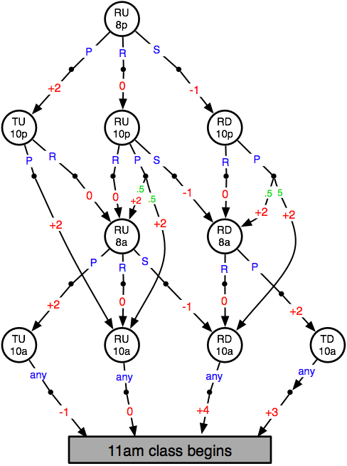
States:
R = RestedT = Tired
D = homework Done
U = homework Undone
8p = eight o'clock pm
Actions:
P = PartyR = Rest
S = Study
any means any action has the same effect
note not all actions are possible in all states
Red numbers are rewards
Green numbers are transition probabilities (all those not labeled are probability 1.0)
The gray rectangle denotes a terminal
state.
Implement a program that models the Party Problem described above. Use any programming language of your choice. Assume that the agent follows a random equiprobable policy (i.e. the probability of picking a particular action while in a given state is equal to 1 / number of actions that can be performed from that state). Run your program for 50 episodes. For each episode, have your program print out the agent's sequence of experience (i.e. the ordered sequence of states/actions/rewards that occur in the episode) as well as the sum of the rewards received in that episode (i.e. the Return with respect to the start state) in a readable form.
What to Hand In (on paper, one copy is sufficient):
- The sequences of experience from each episode, including the Return observed in that episode.
- The values of each state (computed by hand using the Bellman equations).
- The average Return from the fifty episodes.
- The source code of your program.
You may program in any programming language you like, but if you want any help from our esteemed TA, Andrew, it should be one he can read (Python, OCaml, Java, C++, C, Matlab, not Perl). If you'd like to use a language not listed here, please check with Andrew first. Your code MUST be well-formatted and well-documented.
Problems assigned: ex. 2.3, 2.4, 2.5, 2.6, 2.8, 2.16, additional problem (see below).
Additional exercise for Chapter 2 (also due February 14, 2006)
[modified from Rich Sutton's ]
Equation 2.5 is a key update rule we will use throughout the course. This exercise will give you a better hands-on feel for how it works. For this exercise we'll be considering recency-weighted averages of a target signal from time t=0 through time t=15. For all the exercises below, the target signal is: [1, 1, 1, 1, 1, 0, 0, 0, 0, 0, 1, 0, 1, 0, 1, 0]
Get a piece of graph paper (or print this ) and prepare to plot by hand.
(1) Make a vertical axis one inch high that runs from 0 to 1 and a horizontal axis from 0 to 15. Suppose the estimate starts at 0 and the step-size (in the equation) is 0.5. (The estimate should be zero on the first time step.) Plot the trajectory of the estimate through t=15. How close is the estimate to 1.0 after the update at t=4? Suppose for a moment that the target signal continued to be 1.0. Without plotting, how close would it be at t = 10? At t=20?
(2) Start over with a new graph and the estimate again at zero. Plot again, this time with a step size of 1/8.
(3) Make a third graph with a step size of 1.0 and repeat. Which step size produces estimates of smaller error when the target is alternating (i.e., t=10 through t=15)?
(4) Make a fourth graph with a step size of 1/t (i.e., the first step size is 1, the second is 1/2, the third is 1/3, etc.) Based on these graphs, why is the 1/t step size appealing? Why is it not always the right choice?
(5) What happens if the step size is minus 0.5? 1.5? Plot the first few steps if you need to. What is the safe range for the step size?