Here we're using a hypothesized channel model of \(\mathbf{e} \rightarrow \mathbf{f}\), that is \(p(\mathbf{f} \mid \mathbf{e})\). We have a big training set of many \((\mathbf{e},\mathbf{f})\) pairs.
The parameter estimation task is to learn \(\theta\), the translation dictionaries/tables/distributions that parameterize word translations \(p(f_i \mid e_{a_i}; \theta)\). A translation probability is written as \(t(f|e)\). In this document, \(e\) and \(f\) stand for word types, while \(\mathbf{e}\) and \(\mathbf{f}\) stand for sentences (token sequences).
If we had the alignments, we could condition on them and it would be very easy to solve the MLE, by counting pairs of aligned words. Unfortunately we don't have the alignments. They are a latent variable. The correct thing to do would be to sum them out---account for all possible sources the foreign words could have come from---but unfortunately there's no closed form then.
The EM algorithm ("Expectation-Maximization") is a learning algorithm for situations when you want to maximize parameters, but there are latent variables for which if you knew them, it would be easy to maximize the parameters. It turns out Model 1 is a good instance of a statistical model where EM can be applied.
EM can be confusing because it's a very broad class of algorithms, and different sources use the term to mean subtly different things. Model 1 is an instance of a particular variant of EM, which I call Weighting Counting EM. It can be used for models where the complete-data maximum likelihood estimate is based on counting (which is the case here). The algorithm alternates between two steps:
The E-step means "expectation" step, and the M-step means "maximization" step. It turns out that EM eventually converges, and sometimes gives good solutions.
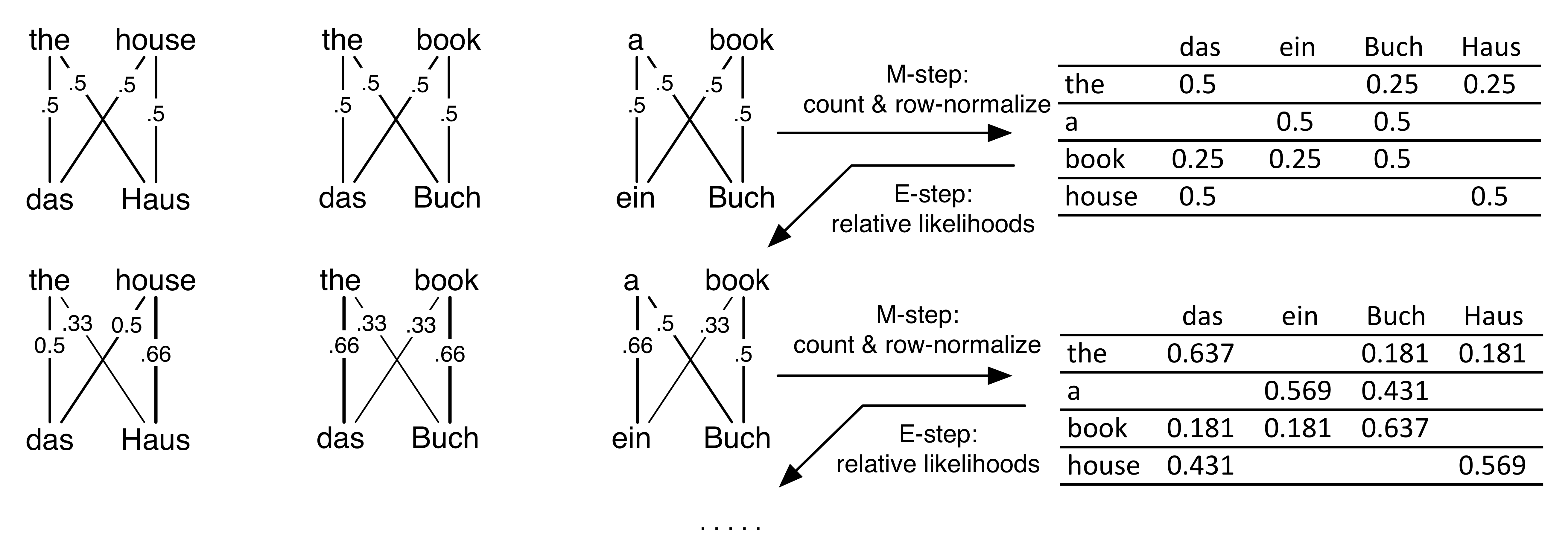
Here's an example. Here there are 4 words in both the foreign and English vocabularies. There are 3 sentences in the training data. Assume no NULLs to make it easier.
Initialize the translation parameters to be uniform. Every row is one \(t(f|e)\) distribution.
| das | ein | Buch | Haus | |
| the | 0.25 | 0.25 | 0.25 | 0.25 |
| a | 0.25 | 0.25 | 0.25 | 0.25 |
| book | 0.25 | 0.25 | 0.25 | 0.25 |
| house | 0.25 | 0.25 | 0.25 | 0.25 |
First E-step: OK, now compute the alignments over the training data.
Why? It's because to figure out your alignment, you look at all the English words you could have come from, and normalize their relative likelihoods. Every word is equally likely to start.
Specifically, for the E-step we need to calculate the posterior probability of every possible alignment variable:
\[p(a_i=j | \mathbf{e},\mathbf{f})\]
For every alignment position \(i\) and possible source \(j\); that is, all \((i,j)\) pairs. It turns out, due to the independence assumption of Model 1, this takes the following form (from page 14 of Collins, which could be derived from the definitions on page 6 or 20), which we then also flip with Bayes Rule,
\[p(a_i|\mathbf{e},\mathbf{f}) = p(a_i | \mathbf{e}, f_i) \propto p(f_i|a_i,\mathbf{e}) p(a_i|\mathbf{e})\]
The second term is constant: \(p(a_i=j|\mathbf{e})=1/l\) for any \(j\) (if we had a NULL, it would be \(1/(l+1)\)), so it can just get folded into the normalizer. Therefore the posterior becomes
\[p(a_i | \mathbf{e}, f_i) = \frac{ p(f_i|\mathbf{e}, a_i) }{ \sum_{j=1}^l p(f_i|\mathbf{e}, a_i=j) } = \frac{ p(f_i| e_{a_i}) }{ \sum_{j=1}^l p(f_i|e_{j}) } \] The first equality is just applying Bayes rule, and the second is just the specific functional forms due to the model. This is an instance of Bayes Rule where the likelihood is the translation model, and the prior is on the alignments. In Model 1, this prior is uniform, so the posterior is just the normalized likelihood. (This corresponds to the \(\delta\) equation on Collins page 20.)
OK, so consider calculating \(p(a_1|\mathbf{e},\mathbf{f})\) on the very first sentence, the alignment for the word das. If it came from the, there's a 0.25 chance it would come out as das, and if it came from house, there's again a 0.25 chance. It's equally likely from either, so either \(a_1=1\) or \(a_1=2\) both have the same 50% posterior probability. That is, \(p(a_1=1|\mathbf{e},\mathbf{f}) = 0.25/(0.25+0.25)\).
In fact, the same thing holds for all the alignment variables everywhere. Therefore all \(p(a_i|\mathbf{e},\mathbf{f})=0.5\).
OK, now time for the first M-step. Let's weighted-ly count how many times \(f\) appears as a translation of \(e\), under the expectations of the alignments. So we just go through every every edge in the diagram above (every \((e_i,f_j)\) pair), and fractionally count that word pair based on the edge's weight, which is the \(p(a_i=j|\mathbf{e},\mathbf{f})\) we just computed in the E-step. To say this mathematically, let \(q_{ij} = p(a_i=j|\mathbf{e},\mathbf{f})\). Then calculate
\[ t(f|e) = \frac{ \sum_{i,j} q_{ij} 1\{f_i=f,e_j=e\} }{ \sum_{i,j} q_{ij} 1\{e_j=e\} }\]
The sums are over all pairs of tokens in the same sentence. The numerator weightedly counts the number of pairs that are word types \(f,e\) (with weights \(q\)), and the denominator sums up all the outgoing edge weights for word \(e\) (no matter what the resulting \(f\) is). (The notation \(1\{...\}\) is the "indicator function", returning 1 if the boolean statement inside is true.)
Thus the following table is the weighted/expected count table for how many times \(f\) was generated by \(e\). All the weights are 0.5 so it's pretty easy to do this by hand here. On the left is the weighted counts table. On the right is after we normalize the rows; thus each row is \(t(f|e)\) for a particular \(e\).
|
→ |
|
Blank cells are zero. Hooray zeros! You get them because alignments can only be within the same sentence. Therefore words that never co-occur in the same sentencepair get zero counts. That's good: we've learned some translations are impossible. Furthermore, not just the zeros; more common co-occurrences, like (the,das), get a higher count than less common ones like (the,Haus). In fact, all this M-step has done is harvest co-occurrence counts from the training data. (We could have used weights 1 for each edge and gotten the same answer... it was just counting.) Anyways, our translation dictionaries certainly seem better than the uniform initialization.
Co-occurrence is a nice intuition, but we can do better with more EM iterations. Now that we have better translation dictionaries, we can better calculate where each word came from. In the second E-step, we compute each of the alignment posteriors again, according to their relative likelihoods from the conditional probability table on the right. The number on each edge is its \(q_{ij}\) posterior prob that \(i\) came from \(j\).
For example: in the second sentence, the Buch-book alignment is 0.66 prob since
\[P(a_2=2|\mathbf{f},\mathbf{e}) = \frac{ t(f_2|e_2) }{ t(f_2|e_1)+t(f_2|e_2) } = \frac{ t(Buch|book) }{ t(Buch|the) + t(Buch|book) } = \frac{ 0.5 }{ 0.25 + 0.5 } = 0.66 \]
Note that \(t(Buch|book)=0.5\), but the probability that in this sentence Buch-book aligns is \(0.66\). That's because \(t(Buch|book)\) is a probability from the translation dictionary. By contrast, the alignment probability is a local probability, specific to just one sentence. Note that in the third sentence, there's another Buch-book pair, but its posterior probability is only \(0.5\), because the "a" competes more strongly as a candidate source. (In real data, we would expect \(t(.|.)\) probabilities to be really small like \(10^{-5}\) or so.)
Count tables are available in in this spreadsheet.