[Intro to NLP, CMPSCI 585, Fall 2014]
Here’s another attempt to explain the EM algorithm for Model 1.
Here I’m using the Collins notation: the translation model is English to Foreign, that is \(\mathbf{e} \rightarrow \mathbf{f}\), that is \(p(\mathbf{f} \mid \mathbf{e})\). We have a big training set of many \((\mathbf{e},\mathbf{f})\) pairs.
The parameter estimation task is to learn \(\theta\), the translation dictionaries/tables/distributions that parameterize word translations \(p(f_i \mid e_{a_i}; \theta)\). For brevity’s sake, sometimes I’ll write a word translation table as \(p(f|e)\). In this document, \(e\) and \(f\) stand for word types, while \(\mathbf{e}\) and \(\mathbf{f}\) stand for sentences (token sequences).
If we had the alignments, we could condition on them and it would be very easy to solve the MLE: \[\max_\theta \sum_{(\mathbf{e},\mathbf{f})} \log p(\mathbf{f} \mid \mathbf{a},\mathbf{e}; \theta)\] This is just estimating a conditional probability based on counting pairs of aligned words.
Unfortunately we don’t have the alignments. They are a latent variable. The correct thing to do would be to sum them out—account for all possible sources the foreign words could have come from—yielding the “incomplete-data likelihood” maximization problem: \[\max_\theta \sum_{(\mathbf{e},\mathbf{f})} \log p(\mathbf{e}|\mathbf{f}) = \sum_{(\mathbf{e},\mathbf{f})} \log\left[ p(\mathbf{e}|\mathbf{a},\mathbf{f};\theta) \times p(\mathbf{a}|\mathbf{f}) \right]\]
The EM algorithm (“Expectation-Maximization”) is a learning algorithm for situations when you want to maximize parameters, but there are latent variables for which if you knew them, it would be easy to maximize the parameters. It turns out Model 1 is a good instance of a statistical model where EM can be applied.
EM can be confusing because it’s a very broad class of algorithms, and different sources use the term to mean subtly different things. Model 1 is an instance of a particular variant of EM, which I call Weighting Counting EM. It can be used for models where the complete-data maximum likelihood estimate is based on counting (which is the case here). The algorithm alternates between two steps:
The E-step means “expectation” step, and the M-step means “maximization” step. It turns out that EM eventually converges, and in fact, it locally optimizes the incomplete-data likelihood maximization problem mentioned above.
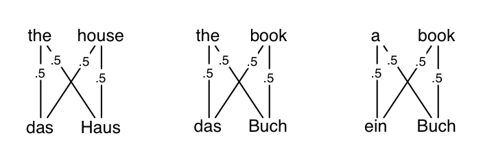
Here’s an example. Here there are 4 words in both the foreign and English vocabularies. There are 3 sentences in the training data. Assume no NULLs to make it easier.
Initialize the translation parameters to be uniform. Every row is one \(p(f|e)\) distribution.
| das | ein | Buch | Haus | |
| the | 0.25 | 0.25 | 0.25 | 0.25 |
| a | 0.25 | 0.25 | 0.25 | 0.25 |
| book | 0.25 | 0.25 | 0.25 | 0.25 |
| house | 0.25 | 0.25 | 0.25 | 0.25 |
First E-step: OK, now compute the alignments over the training data. It will look like this. The alignments’ posterior expectations are all uniform.
Why? It’s because to figure out your alignment, you look at all the English words you could have come from, and normalize their relative likelihoods. Every word is equally likely to start.
Specifically, for the E-step we need to calculate the posterior probability of every possible alignment variable:
\[p(a_i=j | \mathbf{e},\mathbf{f})\]
For every alignment position \(i\) and possible source \(j\); that is, all \((i,j)\) pairs. It turns out, due to the independence assumption of Model 1, this takes the following form (from page 14 of Collins, which could be derived from the definitions on page 6 or 20), which we then also flip with Bayes Rule,
\[p(a_i|\mathbf{e},\mathbf{f}) = p(a_i | \mathbf{e}, f_i) \propto p(f_i|a_i,\mathbf{e}) p(a_i|\mathbf{e})\]
The second term is constant: \(p(a_i=j|\mathbf{e})=1/l\) for any \(j\) (if we had a NULL, it would be \(1/(l+1)\)), so it can just get folded into the normalizer. Therefore the posterior becomes
\[p(a_i | \mathbf{e}, f_i) = \frac{ p(f_i|\mathbf{e}, a_i) }{ \sum_{j=1}^l p(f_i|\mathbf{e}, a_i=j) } = \frac{ p(f_i| e_{a_i}) }{ \sum_{j=1}^l p(f_i|e_{j}) } \] The first equality is just applying Bayes rule, and the second is just the specific functional forms due to the model. This is an instance of Bayes Rule where the likelihood is the translation model, and the prior is on the alignments. In Model 1, this prior is uniform, so the posterior is just the normalized likelihood. (This corresponds to the \(\delta\) equation on Collins page 20.)
OK, so consider calculating \(p(a_1|\mathbf{e},\mathbf{f})\) on the very first sentence, the alignment for the word das. If it came from the, there’s a 0.25 chance it would come out as das, and if it came from house, there’s again a 0.25 chance. It’s equally likely from either, so either \(a_1=1\) or \(a_1=2\) both have the same 50% posterior probability. That is, \(p(a_1=1|\mathbf{e},\mathbf{f}) = 0.25/(0.25+0.25)\).
In fact, the same thing holds for all the alignment variables everywhere. Therefore all \(p(a_i|\mathbf{e},\mathbf{f})=0.5\), which again looks like:
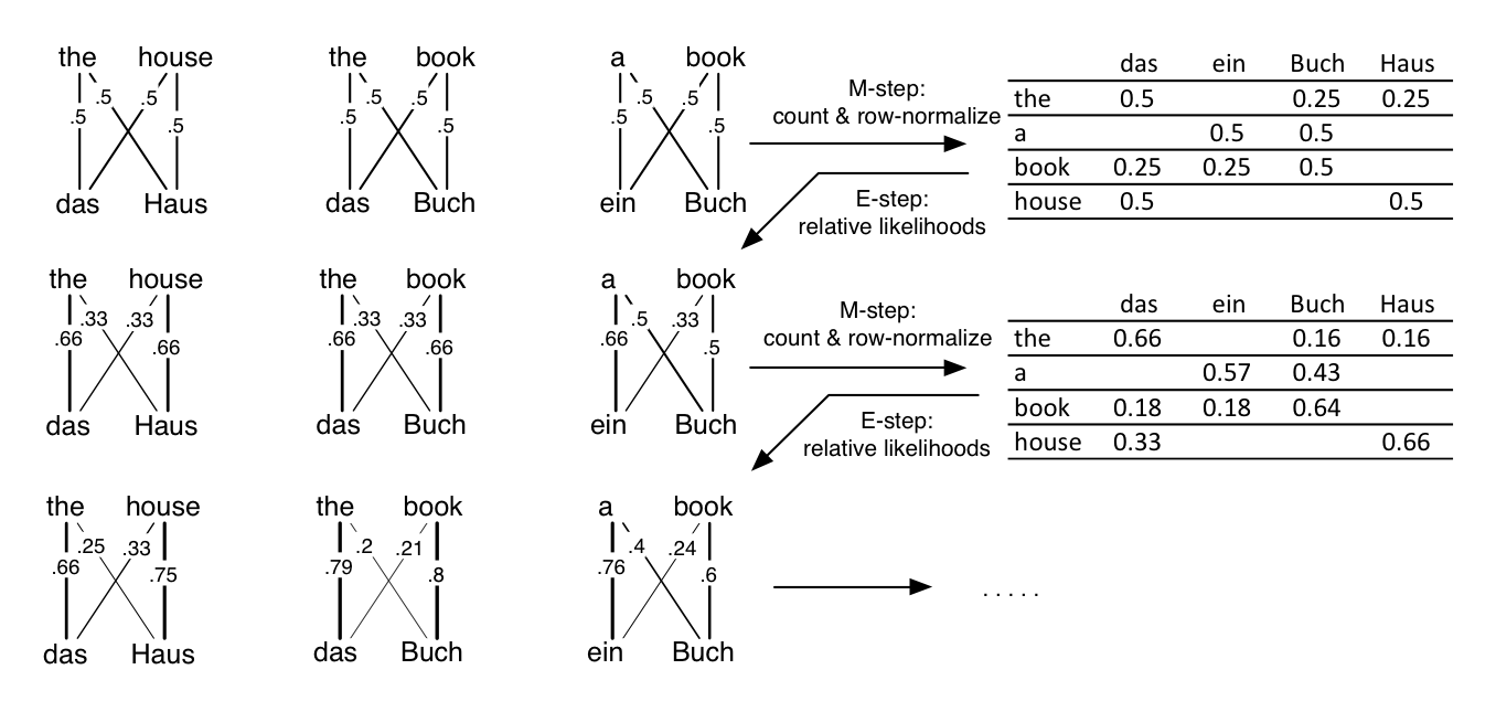
OK, now time for the first M-step. Let’s weighted-ly count how many times \(f\) appears as a translation of \(e\), under the expectations of the alignments. So we just go through every every edge in the diagram above (every \((e_i,f_j)\) pair), and fractionally count that word pair based on the edge’s weight, which is the \(p(a_i|\mathbf{e},\mathbf{f})\) we just computed in the E-step. Thus the following table is the weighted/expected count table for how many times \(f\) was generated by \(e\). All the weights are 0.5 so it’s pretty easy to do this by hand here. On the left is the weighted counts table. On the right is after we normalize the rows; thus each row is \(p(f|e)\).
|
→ |
|
Blank cells are zero. Hooray zeros! You get them because alignments can only be within the same sentence. Therefore words that never co-occur in the same sentencepair get zero counts. That’s good: we’ve learned some translations are impossible. Furthermore, not just the zeros; more common co-occurrences, like (the,das), get a higher count than less common ones like (the,Haus). In fact, all this M-step has done is harvest co-occurrence counts from the training data. (We could have used weights 1 for each edge and gotten the same answer… it was just counting.) Anyways, our translation dictionaries certainly seem better than the uniform initialization.
Co-occurrence is a nice intuition, but we can do better with more EM iterations. Now that we have better translation dictionaries, we can better calculate where each word came from. In the second E-step, we compute each of the alignment posteriors again, according to their relative likelihoods from the conditional probability table on the right. For example, did the first sentence’s das come from the or from house? (Note: the next three sentences have incorrect numbers.) Look at the column for das. It’s twice as likely to be from the versus house. Therefore the posterior weights are \((0.66,0.33)\) for \(p(a_1=1|f,e)\) versus \(p(a_1=2|f,e)\). And so on. (Note: the rest of the document is written assuming this error, sorry!)
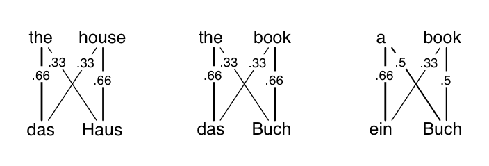
These alignments are better than before. The correct alignments, as you may have guessed, are just vertical ones (these are German phrases with the same word ordering as the English translations). More probability weight is on the correct alignments than before, though it’s still far from correct. Note that Buch in the last sentence is still completely uncertain whether it came from a or book. While it’s the case that Buch co-occurs more with book, the English-side word a appears only once, so in the first M-step after the row-normalization, it was judged to have a sizable potential to become Buch.
OK, so now we keep repeating: weighted counting, normalization for a new translation table, then alignment posteriors based on the translation table, and so on. Here are the alignments and translation tables from the first two EM steps, plus the third E-step. The alignments and translations tables are jointly improving.
Eventually, EM converges, though it’s not guaranteed to converge to the same place from different initializations. Also interesting is a variant of EM called “Hard EM”, where in the E-step, instead of taking the expectation across the posterior, you simply take the most-probable assignment to the latent variable (the most probable alignment). This has the same “chicken and egg” sort of intuitive justification as EM. Hard EM often works less well than EM as we presented here (and, debatably, the theoretical arguments for it are weaker), but sometimes it does work well. There are a zillion other variations of EM as well and lots of study about it, but it’s not well understood exactly when and where it works.
One practical concern with EM for Model 1: you don’t actually have to separate the E-step and M-step as much as was emphasized above. You can make one iteration pass through the data, computing both the alignment posteriors, as well as collecting the weighted counts. Once you’re done passing through the data, you normalize your weighted counts and that’s your new parameter. Once nice thing about this approach is you don’t have to store all the alignment posteriors in memory.
Brendan O’Connor, 2014-09-12
Supporting files: diagram graffle, tables xlsx.